The Liquidity Bible: Part 1

A Primer on Liquidity: Understanding the Invisible Force Behind Market Cycles

Introduction

I still remember the exact moment the Fed announced its unprecedented liquidity measures during the COVID-19 crisis. I was at my trading desk, watching screens filled with red as markets cratered. Investors were panicked, scrambling for safety, dumping stocks, bonds—anything they could sell. The liquidity crisis was unfolding in real time, and then, like a tidal wave, the Fed stepped in. QE, repo operations, corporate bond-buying—whatever it took to stop the bleeding. Within minutes, I saw markets reverse. It was one of those rare moments where you could feel history shift beneath your feet.

That day sparked my obsession with liquidity. I wanted to understand exactly how the Fed’s interventions worked, how liquidity cycles influenced asset prices, and how investors could anticipate these shifts. Over the past few years, I’ve immersed myself in the work of Joseph Wang, who offers unparalleled insights into the Fed’s inner workings, and Michael Howell, who takes a global approach to liquidity. I’ve also had the privilege of discussing these ideas with Andreas Steno Larsen and Oskar Vardål, whose perspectives have sharpened my understanding.

This guide is designed to be the ultimate reference for understanding liquidity—how it works, why it matters, and how it drives financial markets.

Why Should One Care About "Liquidity" in Markets?

The term “liquidity” is often overlooked, yet it profoundly impacts both the way markets work, how asset prices develop over time and where we are in the business cycle. Whether you're trading stocks, bonds, or real estate, understanding liquidity is crucial.

What Exactly Is Liquidity?

In finance, liquidity refers to how easily an asset can be exchanged for cash without significantly affecting its price. For instance, selling an Apple share is far easier than selling a property. Consider this:

• If you owned an Apple share and wanted to sell it, you could likely find a buyer instantly at the click of a button.

• Selling a house, on the other hand, involves listing, marketing, inspections, negotiations, and finding the right buyer—a process that can take weeks or even months.

Liquidity also impacts market efficiency. Another key aspect of liquidity is the bid-ask spread. In highly liquid markets, the spread (the difference between what buyers are willing to pay and sellers are asking) is narrow, ensuring smoother transactions. During a financial crisis, liquidity often evaporates because everyone wants to sell, but few are willing to buy. This causes bid-ask spreads to widen significantly, reflecting the difficulty of executing trades without major price concessions. In such times, liquidity is said to be extremely low.

Defining Global Macro Liquidity

Global macro liquidity can be succinctly described as:

The dynamic ebb and flow of capital across economies and financial markets, shaped by the interplay of monetary policies that determine the expansive or contractive availability of credit and money in the global financial system. This cycle influences investment flows, asset prices, and economic activity.

Liquidity cycles are influenced by monetary policies of major central banks, which dictate when money flows freely or contracts. Sometimes, liquidity drives markets by determining the direction of asset classes. At other times, it operates quietly, like an invisible hand.

Measuring Liquidity

To measure liquidity, we focus on two components:

1. Central Bank Liquidity

2. Money Supply (M2)

1) Understanding Central Bank Liquidity

Let’s analyze the Federal Reserve (FED), the most influential central bank, to understand liquidity concepts.

While the FED sets interest rates, since the 2008 financial crisis, it has employed tools like quantitative easing (QE) to address market turmoil. For example, during the COVID-19 pandemic, even U.S. 10-year government bonds—considered one of the safest and most liquid assets—experienced a spike in bid-ask spreads. In such cases, merely cutting interest rates to zero would not have restored order in sovereign bond markets.

To address this, the FED became the buyer of last resort, committing to buy government bonds and even offering to purchase certain corporate bonds. This intervention calmed markets and re-established confidence. Following the FED’s QE program, asset prices rebounded significantly, with many hitting new highs within six months.

Chart 1.a: Even the World's Most Liquid Asset Can Experience Breakdown

Chart 1.b: Correlation between Fed Liquidity and S&P 500.

How Quantitative Easing Works

To understand QE, we must grasp the role of the FED as the "Bank for Banks."

Key FED Clients

1. U.S. Treasury

   • The FED acts as the fiscal agent for the U.S. government. Tax revenues are deposited into the Treasury’s account at the FED. While the Treasury can draw from this account when needed, it often refrains from using these funds unless absolutely necessary.

2. Primary Dealers

   • These are major financial institutions (e.g., JP Morgan, Goldman Sachs) that have direct accounts with the FED. They enjoy privileges such as borrowing at or near the FED’s target interest rate but must comply with strict capital requirements. Primary dealers also act as intermediaries for the FED, buying assets during QE programs.

3. Other Clients

   • Non-primary commercial banks, money market funds (during market stress), and foreign central banks (via dollar swap lines) also interact with the FED.

The FED’s Balance Sheet

To fully understand monetary plumbing, we need to explore the relationship between movements on the FED’s balance sheet and their corresponding effects on the balance sheets of other entities, such as a major bank (e.g., XYZ Bank). This interplay sheds light on how liquidity is created, transmitted, and utilized in the financial system.

For example, when the FED conducts quantitative easing by purchasing Treasury securities, these assets move onto the FED’s balance sheet as assets. Simultaneously, the reserves of XYZ Bank increase, appearing as a liability on the FED’s balance sheet. For XYZ Bank, these reserves are assets that can be used to support lending, investment, or other operations.

Changes in key components of the FED’s balance sheet—such as deposits, reverse repos, and the Treasury General Account—directly influence the liquidity available to the broader banking system. Understanding these dynamics allows us to trace how monetary policy decisions ripple through the financial system, impacting everything from interbank lending rates to credit availability for businesses and consumers.

The FED’s balance sheet provides insight into its liquidity operations:

1. Assets

   • U.S. Treasury securities (bills, bonds, MBS)

   • Gold and foreign exchange reserves

2. Liabilities

   • Deposits (held by commercial banks)

   • Reverse repurchase agreements (Reverse Repo)

   • Treasury General Account (TGA)

Chart 2.a: FED Balance Sheet

While a bank’s balance sheet looks like this:

1. Assets

   • Loans: The largest portion, representing funds lent to businesses, individuals, and other entities.

   • Reserves: Cash held at the central bank or in vaults to meet regulatory requirements.

   • Securities: Investments in government bonds, corporate bonds, and other financial instruments.

   • Other Assets: Fixed assets, receivables, and miscellaneous investments.

2. Liabilities

   • Deposits: The primary source of funding, which includes customer savings, checking accounts, and term deposits.

   • Borrowings: Funds borrowed from other banks or financial institutions, including interbank loans.

   • Equity: Shareholder capital and retained earnings.

Chart 2.b: Commercial Bank Balance Sheet

Let’s start with Reserves (assets for banks), also called Deposits (liabilities for the Fed).

The saying that the FED can simply "print money" actually refers to its ability to create reserves out of thin air, which can then be credited to the accounts of its clients. As a money-like instrument, banks can use reserves for various purposes. First, as mentioned above, banks are mandated to hold a certain amount of their assets as reserves for security purposes. If a bank has excess reserves or needs reserves to meet daily requirements, it can borrow or lend funds within the overnight interbank loan market (which we will revisit). The key point is that when reserves increase, banks feel wealthier and have more spare capital to seek profitable opportunities, such as creating loans or investing in higher-yielding financial instruments. From thin air, reserves are created, which in turn increases lending and investment activity, thereby boosting liquidity in the market.

The second liability we shall discuss is reverse repurchase agreements, commonly referred to in financial jargon as the Overnight Reverse Repo Program (ON RRP). This is part of the secondary market called the repo loan market (which we will also revisit), where participants who do not necessarily have access to the overnight interbank loan market can borrow or lend funds. A repo is a type of loan in which one seeks cash and pledges a security as collateral. Conversely, a reverse repo is where one lends money in exchange for a security. The borrower of cash pays a small interest when the repo loan terminates and retrieves the collateral posted, similar to a security deposit in case funds are unavailable when the loan is due.

In this framework, the Fed stands ready to borrow excess cash in the system (storing it in the ON RRP account), pledging collateral to entities and promising to return the cash with interest when the repo loan terminates. These reverse-repo loans are typically overnight, meaning each day, cash is posted in this account, and the Fed pays interest on it. The interest rate set here (by the Fed) acts as a floor, as no rational actor would lend at a rate below what the Fed offers. As you might guess, this account removes liquidity from the market by storing cash in the Fed’s vaults, rendering it unavailable for use in financial markets. If cash is abundant in the system and banks have no productive use for it, they replenish the ON RRP account. Conversely, as the liquidity cycle contracts, funds deplete from the ON RRP account, injecting liquidity back into the system.

Chart 3.a: Where Can Excess Liquidity Be Stored When There's Too Much?

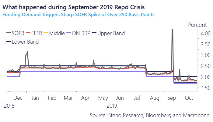
Side Note: Liquidity dynamics often change drastically at and around year-end and quarter-end periods, known as the “window dressing” period. During this time, banks and financial institutions may “dress” their balance sheets for regulatory reporting by shifting from riskier securities to safer ones, creating a heightened demand for cash or cash-equivalent products. This scramble for cash can strain liquidity, affecting the efficiency of the interbank or repo loan markets. (For more details, refer to the 2019 repo crisis.)

Lastly, let’s touch upon the Treasury General Account (TGA), the final liability on the Fed’s balance sheet. As explained earlier, the TGA is where the U.S. government stores its funds. While tax revenues and tariffs contribute to this account, the primary driver of increases in the TGA is government debt issuance through Treasury auctions. When the government decides to build infrastructure, such as a bridge, it issues debt through auctions where primary dealers and other market participants purchase bonds. The proceeds from these auctions are deposited into the TGA account.

A notable scenario arises when the debt ceiling is reached, preventing the Treasury from issuing new debt to fund expenses until Congress approves an increase. In such cases, the Treasury withdraws funds from the TGA to meet spending needs, effectively injecting liquidity into the economy. Conversely, when the TGA is depleted, the government issues new debt to replenish the account, which can negatively impact liquidity.

Chart 3.b: The Treasury General Account & the Impact of the Debt Ceiling

Side Note: The relationship between ON RRP and TGA becomes particularly relevant when the debt ceiling is in effect. During such times, the Treasury cannot issue new debt, leading to a reduction in the availability of Treasury securities. Financial institutions, with fewer options, may park excess cash in the ON RRP account, reducing market liquidity. The net effect depends on the offsetting movements in these accounts, but the overall impact tends to be slightly positive for liquidity conditions.

---

In summary, these dynamics give us a useful equation to understand Fed liquidity:

Fed Liquidity = Total Fed Assets - ON RRP - TGA

---

Chart 4.a: The FED Liquidity Cheat Sheet Formula

Great, now that we have explained the mechanics with regards to fed balance sheet, we can than start questioning how different tools the fed can implement can affect their own balance sheet, banks balance sheet and there effect on liquidity.

Quantitative Easing: When the FED feels like it has no choice but to act as “the lender of last resort”, it will announce to the market how much and how long they will buy bonds. Remember that the FED is suppose to be an independent entity outside from the U.S government. So rather than buy bonds directly from the treasury, it will basically ask Primary dealers to buy any single bonds they can get their hands on and promise them to buy it from them. In exchange like mention, FED will create reserves out of thin air which then banks can use as cash like instruments to go around doing business as usual.

There comes a time when the Fed decides that it’s time to reduce the size of its balance sheet, specifically to unwind the assets it accumulated during the Quantitative Easing (QE) period. This process is called Quantitative Tightening (QT) or balance sheet runoff. While one might assume that the Fed would sell bonds into the market, it typically avoids transitioning from being the largest buyer to the largest seller, as this could disrupt markets. Instead, the Fed opts for a gradual approach by letting its balance sheet "run off."

Chart 4.b: Quantitative Easing (QE) vs. Quantitative Tightening (QT) Cycles

In practice, this means that as bonds held by the Fed mature, it does not reinvest the proceeds into new bonds. This reduces the Fed’s assets as it allows those bonds to expire without replacement. When the Fed’s assets decrease, its liabilities must also decline, which primarily affects bank reserves. From a bank’s balance sheet perspective, this reduction in reserves means that banks have less liquidity available.

However, banks are required to maintain a certain amount of reserves to comply with regulatory requirements. To manage this, banks often turn to their balances in the Overnight Reverse Repo (ON RRP) account as a buffer. By withdrawing funds from the ON RRP account, banks can offset the impact of declining reserves during the early stages of QT. This mechanism helps cushion the immediate effects of liquidity drainage from the system.

As QT progresses and the ON RRP account becomes depleted, banks may have no alternative but to reduce the reserves they hold. This forces banks to curtail their lending and investing activities, as they need to maintain regulatory reserve requirements. With fewer reserves available, banks become more cautious, limiting credit creation and reducing investments in financial instruments. This reduction in lending and investing activity further tightens liquidity in the financial system, amplifying the contractionary effects of QT.

Chart 4.c: Relationship between ON RRP and Reserves

When and why QT ends?

To be able to understand the last and probably the most critical part of QE/QT cycle it is important to go back to 2 markets we referred to above (1) Repo market , (2) Interbank market.

Ever wondered how the Fed manages to keep short-term rates in check? It’s primarily through two key markets: the Interbank & Repo market by setting the (IORB) and the Standing Repo Facility (SRF).

In the Overnight Interbank Loan Market (OILM), the Fed sets a floor for interest rates by offering the IORB. This ensures that no bank would lend reserves at a rate lower than what they can earn by holding reserves at the Fed. On the upper end, the Standing Repo Facility (SRF) provides a cap. It allows banks to access cash by pledging securities, ensuring they can always meet short-term funding needs without driving rates excessively higher.

However, the SRF is rarely used under normal market conditions because tapping it could signal financial distress, creating reputational concerns for banks. Under normal circumstances, most interbank transactions occur at the Effective Federal Funds Rate (EFFR), which typically trades within the range defined by the IORB and SRF.

Chart 5.a: The Interbank Lending Mechanism – How the FED Controls Short-Term Rates

In the Repo Market, the Fed provides a floor through the Overnight Reverse Repo Program (ON RRP), offering the lowest rate one could earn by providing cash. Unlike the Interbank Market, repo markets are collateralized, meaning every loan must be backed by a security of equal or similar value. Normally, the Fed sets the lower bound of the repo market either at or slightly above the floor in the interbank market to ensure a stable and predictable interest rate environment. On the other hand, the Fed can also provide cash through the Standing Repo Facility (SRF) to institutions in dire need. Yet again, this facility has not been widely used, as market participants aim to avoid unnecessary signaling.

Chart 5.b: The Repo Lending Mechanism – How the FED Controls Short-Term Rates

Under normal circumstances, most transactions in the repo market occur at the Secured Overnight Financing Rate (SOFR), which typically trades within the range defined by the ON RRP and SRF.

There comes a time, at and around the end of the liquidity cycle, when money becomes extremely tight. It becomes increasingly difficult to secure funding in both the interbank and repo markets. Lenders of cash grow reluctant to lend, as they may need the liquidity themselves, while borrowers grow anxious about meeting their liquidity needs but avoid seeking assistance from the Fed through the SRF due to the negative signaling this would send. Signals of stress often emerge first in the repo market, where SOFR begins to trade above and beyond the upper bound.

Side Note: Why do we see SOFR spikes before the Fed funds rate, especially during window dressing periods? Remember that repo rates are largely market-driven. During these periods, financial institutions need to hold High-Quality Liquid Assets (HQLA), such as treasuries, to meet specific liquidity coverage ratios. While some participants are willing to provide cash, they often require HQLA as collateral in exchange. This creates a shortage of HQLA while simultaneously increasing demand for cash. As a result, the interest rate participants are willing to transact at rises, causing SOFR to spike. This mismatch between HQLA availability and cash demand drives the temporary increase in SOFR during these periods.

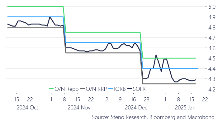
Chart 5.c: What Happens When the FED Loses Control of Interest Rates?

Side Note: What might the Fed try to do in order to continue QT for slightly longer? The Fed might employ technical methods to mitigate the apparent stress signaled by the funding market, thereby extending rounds of quantitative tightening. One approach has been to lower the ON RRP rate by 5 basis points closer to the IORB bound. By doing so, the Fed could encourage participants with money parked at the Fed (ON RRP) to deploy it back into the financial system, providing a brief liquidity cushion. However, this strategy primarily serves to reduce sudden attention on the stress signals without addressing the underlying issues.

Chart 5.d: FED Tactics to Manipulate Market Mechanics

Side Note: When should we worry about the level of reserves within the system? One of the most critical questions the Fed faced during the last QE cycle was whether there is a specific equilibrium level of reserves that should not be breached. It is important to remember that QE and QT are relatively new tools for the Fed, and the central bank is still navigating this experimental territory.

During the last cycle, the equilibrium level of reserves appeared to be around $1.5 trillion. Banks became accustomed to this level of reserves post-QE, as it provided a foundation for extending credit and loans, albeit with lowered lending standards. At the same time, banks pursued riskier investments to compete in higher-yielding markets. QE inherently increases the level of risk-taking by financial institutions because of the surplus liquidity it creates.

However, the idea of a fixed equilibrium level for reserves is flawed. As each QE cycle progresses, a new equilibrium emerges, reflecting the adjusted behavior and expectations of banks and financial institutions. Currently, the new equilibrium for reserves seems to be around $3 trillion. Funding signals already indicate that liquidity is extremely tight, as evidenced by the near-depletion of the ON RRP account. This drawdown has cushioned the decline in reserves thus far, suggesting that banks are still relying on this buffer. However, we are now seeing SOFR trade outside its typical range, signaling stress in funding markets even before reserves have significantly fallen. This indicates that banks may soon face greater pressure to reduce reserves, which could lead to a contraction in the availability of loans and credit.

When funding needs are at the largest and the Fed is out of the tool it can employ to prevent further spikes, it has not other choice but to end their quantitative tightening program. This marks the end of the FED liquidity cycle.

Chart 5.e: When Do Reserves Start to Become Scarce?

Great! Now that we have a decent understanding of how Fed liquidity works, the next component to analyze is the Money Supply.

2) Understanding Money Supply Liquidity

You might have come across the term "money supply" in an economics class. It’s a broader metric that essentially measures the amount of money circulating in the economy, and it’s constantly changing. Money supply is typically broken down into four categories:

• M0: The most liquid form of money, consisting of cash and coins in circulation.

• M1: Includes M0 plus demand deposits, such as checking accounts and other liquid assets.

• M2: Expands on M1 by including savings accounts, money market funds, and time deposits under $100,000.

• M3: The broadest measure, incorporating M2 as well as larger time deposits, institutional money market funds, and other larger liquid assets (though not always reported in some countries).

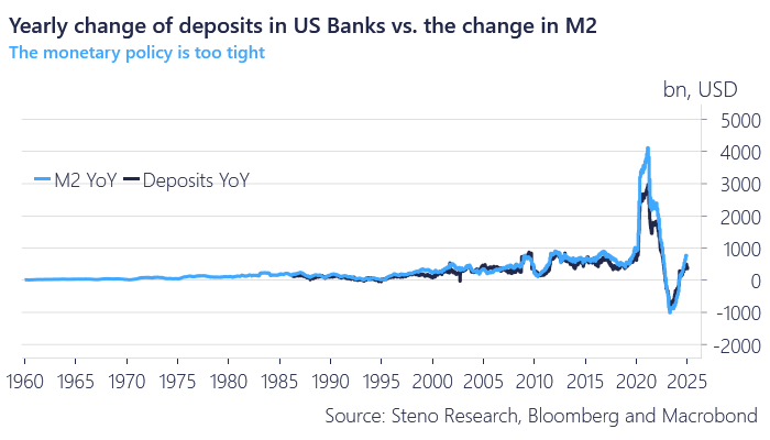
While access to detailed data for these categories varies by country, they generally move in tandem. So, focusing on one metric, such as M2, can provide a good sense of money creation within a country's monetary system. Broadly speaking, when M2 is rising, there’s likely more liquidity in the system—more loans, savings, bank deposits, and central bank money flowing through the economy.

Chart 6.a: Money Supply vs S&P 500

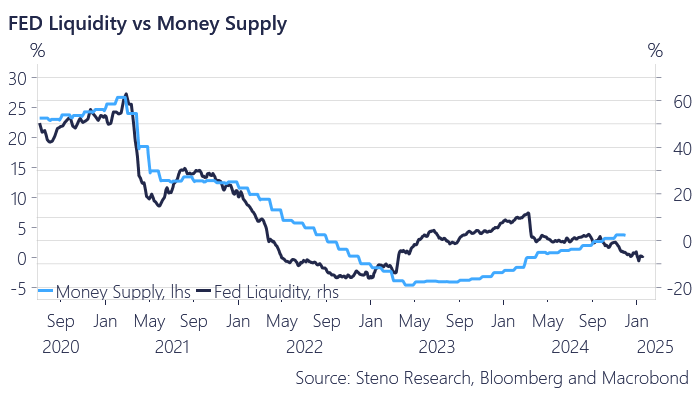
Fed Liquidity vs. Money Supply: Why They Can Diverge

Although central bank liquidity is a major driver of the money supply, there are cases where the two can diverge. This is especially apparent during different phases of the Fed’s monetary policy cycles:

1. The Start of a QE Cycle

   • At the beginning of quantitative easing (QE), the Fed creates reserves by purchasing assets (like Treasuries or mortgage-backed securities) from the financial system. This injection of liquidity boosts the money supply because banks have more reserves to either lend out, fueling credit creation and economic activity and buying securities.

2. During Balance Sheet Runoff (QT)

   • As the Fed begins to unwind its balance sheet through quantitative tightening (QT), it reduces its assets and removes liquidity from the system. However, the economy doesn’t experience an immediate decline in money supply because reserves are already so abundant that banks can continue to lend and invest in the broader economy. In essence, the "trickle-down" effect of earlier QE cycles allows the money supply to keep growing, even as Fed liquidity declines.

3. Demand for Loans and Credit Spreads

   • QE is not only about providing liquidity—it’s also designed to stimulate the economy. Lower interest rates and tighter credit spreads encourage borrowing and investment, driving up loan demand. Even as the Fed tightens, banks may still see strong incentives to lend, sustaining M2 growth.

4. The Role of the Yield Curve

   • Another key factor influencing the money supply is the shape of the yield curve. When the curve steepens, the spread between short-term borrowing costs and long-term lending rates widens. This increases profitability for banks, incentivizing them to lend more. As a result, a steep yield curve can accelerate deposits which increase money supply growth.

5. Economic growth: If the economy surprises to the upside, that means that incomes, spending and investment remains high, which would lead to more loans and deposits, overall increase M2.

6. Bank capital requirements: changes in bank requirements significantly influence the money supply by altering banks' ability to lend. For instance, stricter reserve or capital requirements reduce the amount of funds banks can use for lending, effectively decreasing the money supply by limiting the creation of new deposits through the credit multiplier effect. Conversely, easing these requirements—such as during economic downturns—frees up bank resources, encouraging lending and increasing the money supply as loans generate new deposits. The Federal Reserve, through tools like reserve requirements and stress testing, uses these levers to control liquidity and stabilize the economy, directly impacting the availability of money circulating in the financial system.

   Chart 6.b: More Money in Vaults Leads to Greater Capital Deployment

   

Side Note: What is Basel III and how did it affect bank requirements? Adopted in 2010 after the 2008 financial crisis, Basel III introduced stricter rules to strengthen bank resilience. It focuses on:

1. Capital Requirements: Higher quality capital (e.g., CET1) ensures banks can absorb losses during crises.

2. Liquidity Standards: Rules like the Liquidity Coverage Ratio (LCR) and Net Stable Funding Ratio (NSFR) ensure banks can meet obligations without selling assets quickly.

3. Leverage Ratio: A 3% minimum cap limits excessive borrowing, adding a safety net.

These measures impact M2 (money supply) by regulating lending. Stricter rules can slow credit creation and reduce M2, while relaxed measures during crises can boost lending and expand M2.

Chart 6.c: Overlaying Both Metrics on a Single Chart for Comparison

Conclusion

Taken from The Big Short, the image above captures a blunt but insightful truth: most people hate poetry, just as most traders ignore the complexities of liquidity—until it’s too late. But those who truly understand it can gain a significant edge.

The inner workings of liquidity are often overlooked because they seem boring—and in many ways, they are supposed to be. However, in financial markets, liquidity is one of the most important yet least appreciated factors. Much like in a high-stakes poker game, those who understand the mechanics behind liquidity have a strategic advantage over those who don’t.

As my finance teacher used to say, the financial market is an arms race—those with the bazookas will always overpower those with pistols. This is why knowledge is key. The ability to understand how liquidity moves, who controls it, and when it dries up can mean the difference between surviving a market downturn and being wiped out entirely. Hopefully, this primer has provided you with a few valuable insights into these dynamics.

This "Bible" of liquidity should be something you carry with you—figuratively, if not literally. Understanding liquidity allows for better, more precise decision-making and risk management. It’s not just another factor to consider; it’s the foundation upon which market stability, volatility, and opportunity rest. Liquidity MATTERS.

I hope this piece provided value and sparked new ways of thinking. It took time and research to put together, and if you found it insightful, I’d appreciate it if you liked it, restacked it, or shared it with friends and colleagues. The more people understand liquidity, the better prepared they’ll be to navigate the financial battlefield.

Until Next Time…

Sam

Please note that the content provided above is for informational purposes only and should not be considered financial advice. Always conduct your own research and consult with a qualified financial advisor before making any investment decisions.